From the moment the SD/SDXL was unveiled, the pace of advancements in image generation never stops. Almost every day, the open-source community rolls out novel techniques that enhance the pipeline’s aesthetic appeal and versatility. Yet, many of these innovations lack detailed documentation or in-depth explanations. To learn these tricks, one has to spend hours reading through the source codes. To simplify this process for developers and provide a convenient reference, I’ve written this blog to collect the tricks that lie beneath the published and source codes.
Artistic Respect and Recognition: All artworks referenced in this blog are attributed to their original creators. Images inspired by these artists’ unique styles are not permitted for commercial use. If you create an image by referring their art style, please kindly give credit by acknowledging the artist’s name.
SDXL Architecture
In the SDXL paper, the two encoders that SDXL introduces are explained as below:
We opt for a more powerful pre-trained text encoder that we use for text conditioning. Specifically, we use OpenCLIP ViT-bigG in combination with CLIP ViT-L, where we concatenate the penultimate text encoder outputs along the channel-axis. Besides using cross-attention layers to condition the model on the text-input, we follow and additionally condition the model on the pooled text embedding from the OpenCLIP model.
To clarify how the two text encoders work together, here is a diagram I’ve made to illustrate the pipeline.
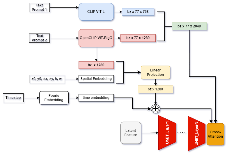
Figure 1. text encoder pipeline in SDXL; text_prompt 1 and text_prompt 2 are two prompts, which can be different; x0, y0, ∆x, ∆y, h, w are 6 spatial conditions newly introduced by SDXL
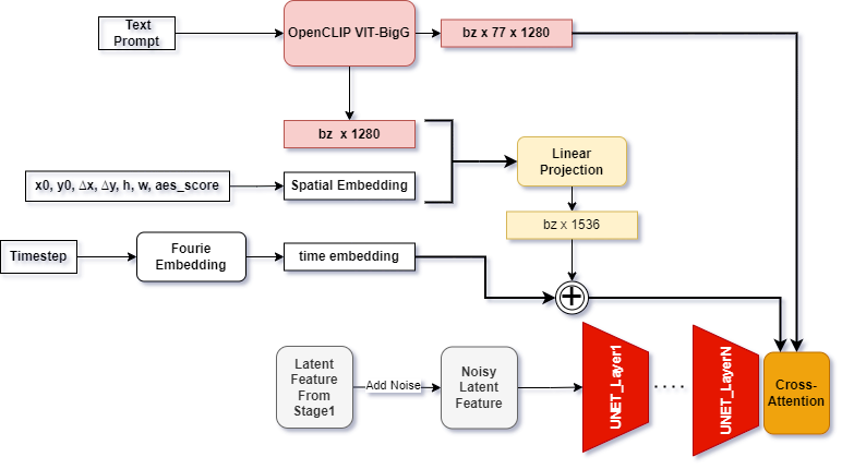
Figure 2. SDXL Refiner pipeline; x0, y0, ∆x, ∆y, h, w, aes_score are spatial conditions and aesthetic score introduced to guide the image generation
SDXL also has a refiner stage. Specifically, it is implemented as an img2img pipeline. While the paper may not explicitly mention it, it’s essential to note that the refinement stage takes aesthetic scores as a guiding factor besides the coordinates and image sizes. Specifically, a positive aesthetic score of 6.0 and a negative aesthetic score of 2.0 are used as the thresholds, which means that we expect the SDXL refiner will produce images with an average aesthetic score exceeding 6.0.
It’s interesting to notice that the 768-dim hidden features from the smaller text encoder are directly concatenated to the 1280-dim hidden features of the larger text encoder. Note that text_prompt_1 and text_prompt_2 can be different. Given the intuition that higher dimensions can capture fine-grained features, some AI painters prefer to feed style descriptions into CLIP-ViT-L and prompts about body motion, clothes, or facial expressions into the other text encoder. Additionally, it’s worth noting that the pooled feature from the larger text encoder acts as a bias to adjust the time embedding
Below are the visualization about the SDXL/SDM UNet structure. These are two graphs I always come to check out
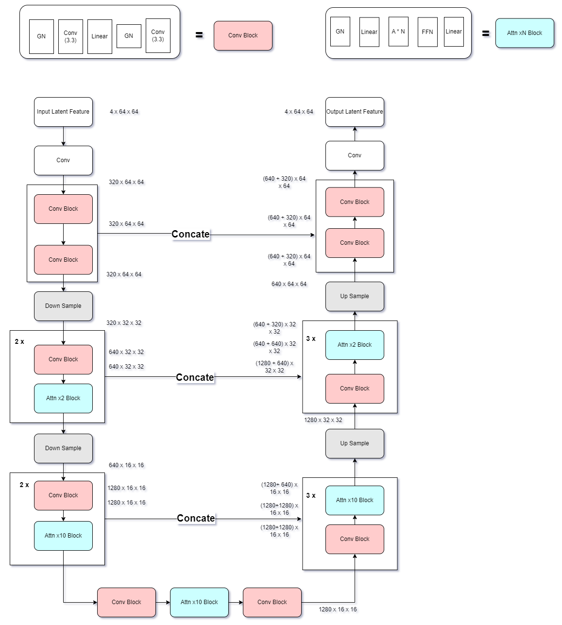
Figure 3. SDXL UNET structure
Compared SDXL UNET with SDM UNET,
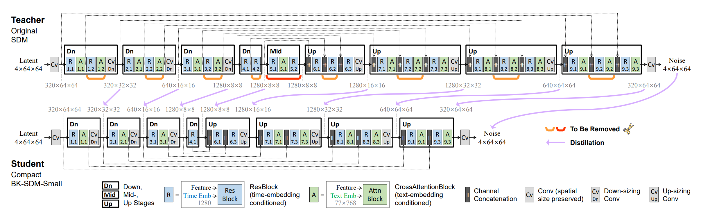 Figure 4. Original SDM UNET structure; image credited to BK-SDM paper
we can clearly see from Fig.3 and Fig.4 that the lowest latent dimension is set to 16 rather than 8. According to the paper, they remove the dimension 8 for computation efficiency. Moreover, they also omit the transformer block at the highest feature level, further saving the computation cost.
Reference-only Mode
Reference-only mode is one of my favorite features in the SD pipeline, which enables art style transfer from a reference image to a new image based on a given prompt, without training.
It is first introduced by lllyasviel in this discussion thread.
Here is a showcase from this reference only.

Figure 5. A reference-only showcase; Left: reference image credit to @001_31_; Right: generated image; We can clearly see the generated image “plagiarizes” the art style of the reference image like colors, lines and character face; please check the appendix for generation setting.
The idea behind the reference-only is quite straightforward. It requires running the diffusion process twice. In the first round, the VAE encoder encodes the reference image into a latent feature, termed as \(x_{ref}\). This reference latent feature is then interpolated with a randomly initialized latent feature. We denote the noisy latent feature as \(x\).
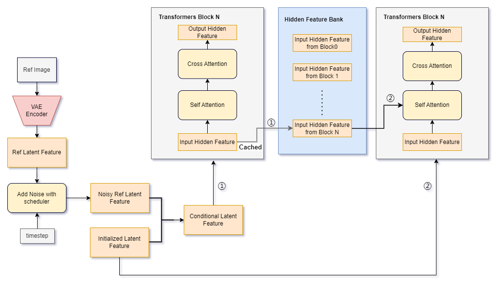 Figure 6. reference-only pipeline; ①: the first diffusion forward pass, ②: the second diffusion forward pass
Suppose we are playing this reference-only mode with an SD1.5 checkpoint. As we know, SD1.5 has 16 TransformerBlocks across all UNet layers. Therefore, during the first diffusion forward pass, 16 hidden features are generated and stored in the memory band. Subsequently, we pass \(x\) to the second diffusion forward pass.
The self-attention block uses the previously cached features from the corresponding Transformer Block layer in the prior diffusion as a reference clue. In other words, there are now “two” cross-attention blocks in the second diffusion forward pass. One is conditioned on the reference clues generated from \(x_{ref}\), while the other is conditioned on the text features.
As for the self-attention part in the second diffusion forward pass, There exist implementation variants that can yield different generation outcomes.
In the following discussion, we denote the input features of the self-attention block as \(h_{in}\) within one TransformerBlock, and the resulting feature as \(h_{out}\). Typically, we apply the classifier-free method for text guiding, \(h_{in}, h_{out} \in \mathbb{R^{2 \times N \times dim}}\), where \(N\) is the number of elements in the latent feature, \(dim\) is the hidden feature dimension.
Additionally, we denote the cached features from the same TransformerBlock generated in the first diffusion forward pass as \(h_{cond} \in \mathbb{R^{2 \times N \times dim}}\)
Reference-fine-grained
One implementation is only the conditioned latent features use the cached features as the cross-attention clue, while the unconditioned latent features compute cross-attention itself. The pseudo-code is provided below:
attn_output_uc = attn( h_in,
                       encoder_hidden_states=torch.cat([h_in, h_cond] , dim=1))

attn_output_c =  attn( h_in[0], encoder_hidden_states=h_in[0])

h_out = style_fidelity * attn_output_c + (1.0 - style_fidelity) * attn_output_uc
This is how huggingface implements. check the code here.
I’d like to refer it as reference-fine-grained
Reference-coarse
Another implementation processes both the unconditional and conditional latent features in the same way. I prefer to call it reference-coarse
h_out = attn( h_in,
              encoder_hidden_states=torch.cat([h_in, h_cond], dim=1))
Reference-adain
reference_adain is another mode proposed by lllyasviel, who drew inspiration from the paper, “Arbitrary Style Transfer in Real-time with Adaptive Instance Normalization”. AdaIN, short for Adaptive Instance Normalization, works on a premise: when given content input \(x\) and style input \(y\), the style transfer can work by aligning the channel-wise mean and variance of \(x\) with those of \(y\).
In the reference_adain mode, not only are the input hidden features sent to the Transformer Block, but the mean and variance of these features are also cached during the first diffusion forward. Additionally, the mean and variance of the output features of the ResNet Block in the UNet stage without a Transformer, are stored as well. During the second diffusion pass, these stored values are applied to adapt to respective hidden features from the same blocks.
Reference mode comparsion
The modes mentioned above can work together. Figure 6 compares the generation output in different reference modes.
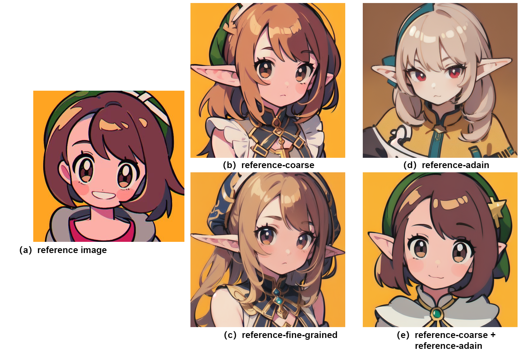 Figure 7; reference mode comparison. All images are generated with the same setting. For setting details, please check the appendix (a): a reference image credit to @001_31_; (b) reference-course; (c) reference-fine-grained; (d) reference-adain; (d) combine reference-course and reference-adain;
From (b) and (c), we can see there are fine-grained added elements in (c) not present (b), such as the decorations on the character’s hat and the detailed hair strands; (d) shows that the reference image in reference-adain offers limited guiding to the final output. Notably, the colors of the character’s hair, background, and eyes are quite different from those in (a); From (b) and (e), we can find the reference-adain can help the generation closely align to the style of the reference image, such as the character’s face, hat, face angle, coloring style. Instead, reference-course enables the pipeline paint more freely, using the reference only as a loose guide.
I recommend playing with these reference mode combinations to discover your favorite settings.
Slider LoRA
This innovative method offers the flexibility to seamlessly modify the body/concepts of your character, much like using a slider to customize your character in a video game. Moreover, it ensures character consistency without the need for cumbersome prompt engineering and random attempts. While the community hasn’t agreed on how to name it, some suggest “negative LoRA” as a counterpart of “negative embedding”. However, Since I first learned about it from this awesome post by エマノン, I’ve chosen to follow his terminology, dubbing the technique “Slider LoRA”.
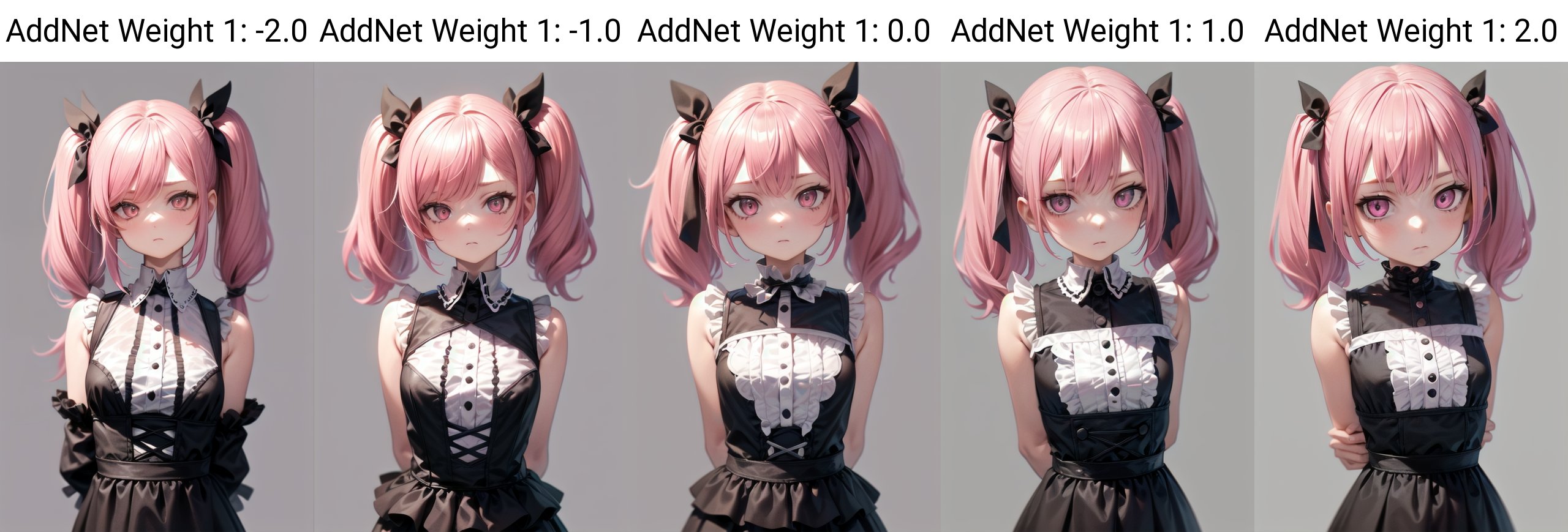 Figure 8; A showcase of slider LoRA, which can adjust the head size of the character with character consistency; credit to @Emanon_14
エマノン さん’s post introduces how to create a Slider LoRA. For those who don’t read Japanese, I’ve summarized the key points from the original post below.
エマノン さん proposes two approaches to making a slider LoRA based on コピー機学習法 (copy machine learning).
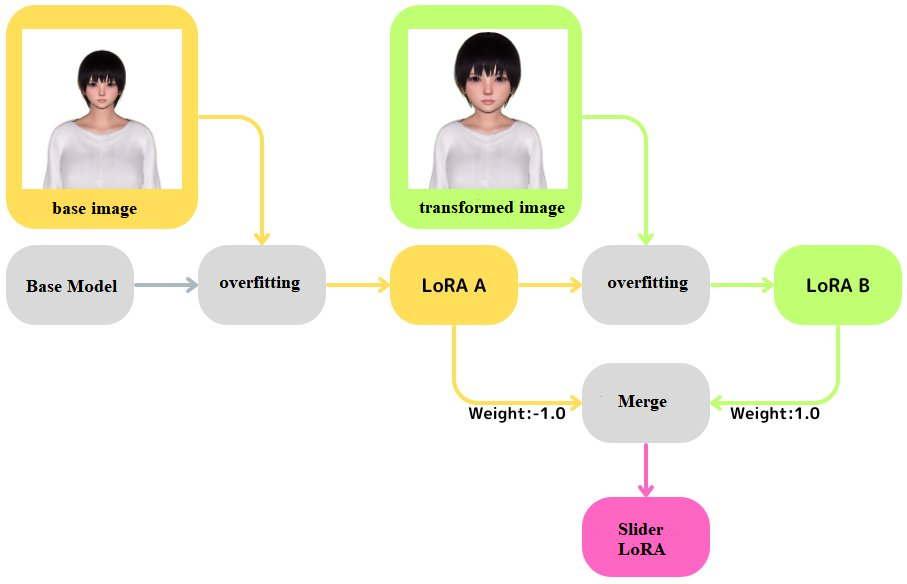
Figure 9; First, merge a LoRA, which is overfitted to one reference image, into the base mode. Then, merge another LoRA, overfitted an image transformed from the previous one, into the merged model; credit to @Emanon_14
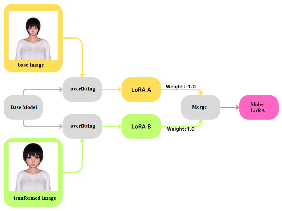
Figure 10; Merge LoRA A, which is trained to overfit one reference image, and LoRA B, which is trained to overfit another image, into the based model using different weights; credit to @Emanon_14
According to the post, copy machine learning is a parameter-efficiency training method. To be specific, it leverages LoRA on the transformers block in the UNet, then overfits it until the model can reconstruct the training image with an empty prompt.
In the following training pipeline, we take the second approach as an example
Prepare the Training Dataset
The training data is organized in pairs. These paired datasets differ in specific angles, with each pair varying only in the concept that you want the LoRA slider can recognize. For example, here is a training pair only different in the head size of the character.
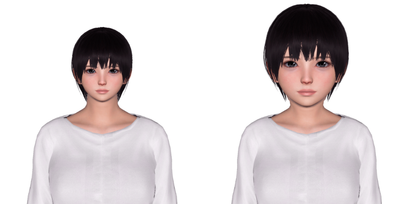
Figure 11; credit to @Emanon_14; Except for the head size of the two characters, the other components remain identical at the pixel level.
Copy Machine Learning
Next, let’s train two UNet LoRAs, using images from each set, for about 1000 ~ 3000 steps.
When the LoRA can replicate the original training image using an empty prompt, we can say the training is successful. Empirically, the optimal LoRA rank dimension is 4 ~ 16.
Merge the LoRAs
Finally, it’s time to merge two LoRAs that memorize opposite concepts into one LoRA. This merging is realized by svd_merge_lora method.
The idea of svd_merge_lora is straightforward, It first merges two LoRA weights into the base model. Then, it leverages Singular Value Decomposition (SVD) on the merged weights to derive the final LoRA. Notably, the rank dimension of the final LoRA derived with SVD is usually double that of the initial LoRA weights.
Appendix
1. the generation setting of Figure 5 (reference-only showcase)
-
prompt: masterpiece,best quality, ultra highres, detailed illustration, portrait, detailed, girls, detailed frilled clothes, detailed beautiful skin, face focus
-
negative embedding: EasyNegative, bad-picture-chill
-
sd1.5 checkpoint: A fine-tuned checkpoint based on SD1.5 with proprietary dataset
2. the generation setting of Figure 7 (reference mode comparsion)
-
prompt: masterpiece, best quality, 1girl, medium hair, elf, pointy ears, loli, teen age, looking at viewer, :3
-
negative embedding: EasyNegative, bad-picture-chill
-
sd1.5 checkpoint: A fine-tuned checkpoint based on SD1.5 with proprietary dataset