Translated from the post, originally written in Chinese by Su, Jianlin
Translated by Norm Inui
TL;DR
- Interpret RoPE from the perspective of a β-based encoding.
- Introduce recent developments in the open-source community regarding long contexts.
- Some approaches, such as NTK-aware Scale RoPE, can extend context length without fine-tuning.
For developers who are interested in how to extend the context length of LLMs (Large Language Models), the open-source community has continuously presented us with fascinating methods in the past few weeks. First, @kaiokendev experimented with a “positional linear interpolation” approach in his project SuperHOT.
He demonstrated that with minimal fine-tuning on long texts, existing LLMs can be easily adapted to handle contexts over their pretraining context length. Almost simultaneously, Meta proposed the same idea in the paper titled “Extending Context Window of Large Language Models via Positional Interpolation.”
Shortly after the paper was published, @bloc97 introduced the NTK-aware Scaled RoPE, enabling LLM to extend its context length without fine-tuning! With all these methods, especially the NTK-aware Scaled RoPE, it persuades me to revisit the idea behind RoPE from a \(\beta\)-based encoding perspective.
Encoding the Number
Suppose we have an integer \(n\) within \(1,000\) (not including \(1,000\)) that we want to input into a model. What would be the best way to do this?
The most intuitive idea is to input it directly as a one-dimensional vector. However, the value of this vector has a large range from \(0\) to \(999\), which is not easy to optimize for gradient-based optimizers. What if we scale it between 0 and 1? That’s not good either, because the difference between adjacent numbers changes from \(1\) to \(0.001\), making it challenging for both the model and optimizer to distinguish between the numbers. In general, gradient-based optimizers are a bit “vulnerable” and can only handle inputs that aren’t too large or too small.
To solve this problem, it is necessary to find a smart way to represent the input. We might think about how we humans do. For an integer, like \(759\), it’s a three-digit number in decimal, with each digit ranging from 0 to 9. This inspires me to represent the input in decimal directly as a vector. That is, we transform the integer \(n\) as a three-dimensional vector \([a,b,c]\), where \(a\), \(b\), and \(c\) represent the hundreds, tens, and units of \(n\) respectively. By increasing the input dimension, we can both reduce the range of each digit and get rid of small resolution between numbers. Luckily, neural networks are good at handling high-dimensional vectors.
If we want to further reduce the value span of each dimension, we can simply decrease the base, like using 8, 6, or even 2 as the encoding base at a cost of an increase in input vector dimensions.
Let’s say we have trained a model with the input ranging from \(0\) to \(999\) represented as a three-dimensional vector in decimal. Then we want to enlarge the upper bound of \(n\) from \(1,000\) to \(2,000\). How can we realize this?
If we follow the same idea discussed above, the input will now be a \(4\)-dimensional vector. However, the model was trained for a \(3\)-dimensional vector. Therefore, the input with an extra dimension may confuse the model. Some might wonder why can’t we reserve extra dimensions in advance? Indeed, we can pre-allocate a few more dimensions. During the training phase with the upper bound as \(1,000\), they can be set to \(0\), but during the inference phase with an upper bound as \(2,000\), the pre-allocate dimension has to be set to value besides \(0\). This is what we call Extrapolation.
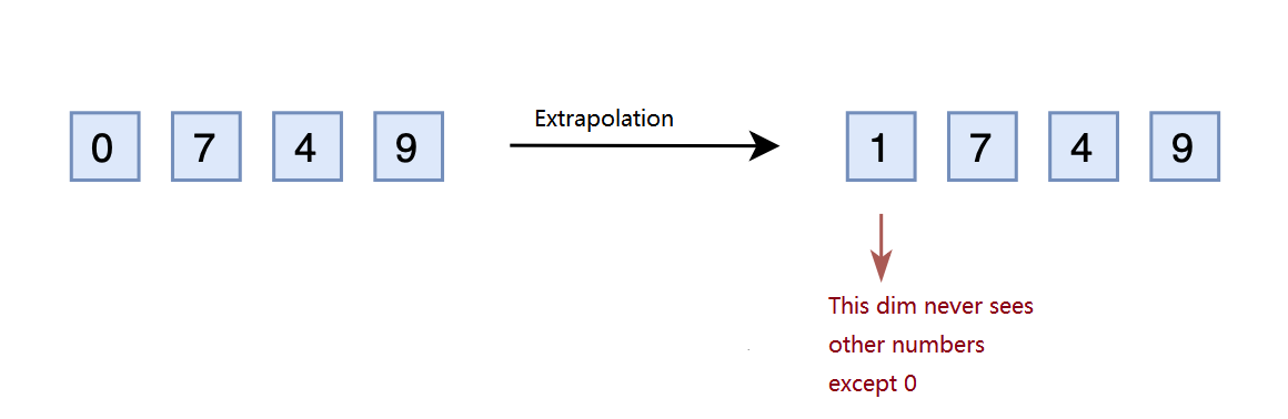
However, the dimensions reserved during the training phase have always been set to \(0\). If these dimensions were changed to other values during the inference phase, the performance might be significantly harmed. This is because the model is never trained to adapt to those pre-allocated dimension in different values.
Linear Interpolation
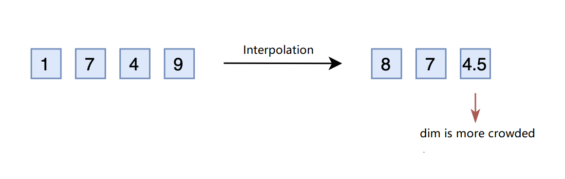
Considering the challenges above, some proposed interpolation instead of extrapolation to compress the value upper bound of \(2,000\) down to \(1,000\). For example, the number \(1749\) can simply compress to \(874.5\) by dividing \(2\). Thus, \(874.5\) can be converted into a three-dimensional vector \([8,7,4.5]\). Following this double mapping strategy, the vector \([7,4,9]\) now corresponds to \(1498\).
However, the difference between adjacent numbers was \(1\), but now it is \(0.5\), making the last dimension more “crowded”. Therefore, interpolation usually needs to fine-tune the model to make it adapt to the “crowded” dimensions.
You might notice that the extrapolation can also be fine-tuned to adapt to the pre-allocated dimension. Well, that is correct, but the interpolation requires far fewer steps compared to extrapolation. It is because position encoding (both absolute and relative) has taught the model to understand the relative concept rather than precisely knowing what the number it is, that is: the model knows \(875\) is greater than \(874\), but it doesn’t know what is \(875\).
Given the generalized ability of LLM, injecting the concept that \(874.5\) is greater than \(874\) is not particularly challenging.
However, this interpolation approach is not without flaws. The broader the range we want to expand, the smaller the unit dimension resolution becomes, while the hundreds and tens dimensions still remain at a resolution of 1. This means that the interpolation implicitly introduces resolution inconsistency across dimensions. Each dimension is not equally interpolated, making fine-tuning/continuing learning challenging.
Base Conversion
Is there a method that doesn’t require adding extra dimensions and can still maintain resolution across dimensions? The answer is YES.
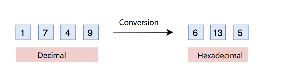
It is a solution that we are all familiar with, base conversion. A three-digit decimal number can represent \(0\) to \(999\). What if it’s in hexadecimal? Its maximum value in 16-base can be \(16^3-1=4095 > 1999\). So, by simply converting to hexadecimal, with a base of 16, such as turning \(1749\) into \([6,13,5]\), a three-dimensional vector can represent a larger range. The cost? Each dimension’s value changes from a range of \(0-9\) to \(0-15\).
It’s indeed a clever idea. As mentioned earlier, what we care about is relative position information in the sequence since a trained model has already learned \(875 > 874\). This holds true in hexadecimal as well. The model doesn’t care what base you use to represent the input, but only the relative information. Now, the only problem would be if the value of each dimension exceeds \(9\) (values between \(10-15\)), will the model still know how to compare accurately? Luckily, most LLMs have such capability. Based on this hypothesis, we can now extend the range without fine-tuning! Furthermore, to make interpolation more robust, we can use a smaller base like \(\lceil\sqrt[3]{2000}\rceil = 13\) instead of \(16\) to limit the value range of each dimension.
This idea of base conversion finally leads us to the NTK-aware scaled RoPE that was mentioned at the beginning.
Positional Encoding
Based on the explanation above, we can claim:
The Rotational Positional Encoding (RoPE) at position \(n\) is the \(\beta\)-based encoding of the number \(n\)
This might surprise you at first glance, however, it does hold true.
Proof:
Suppose we have a decimal number \(n\). To calculate the digit at position \(m\) (counting from right to left) in its β-based encoding, we have:
\[\begin{equation}\lfloor\dfrac{n}{\beta^{m-1}}\rfloor \mod \beta \end{equation}\]
As for RoPE, which is adapted from Sinusoidal Position Embedding
\[\begin{equation}[\text{cos}(\dfrac{n}{\beta^0}), \text{sin}(\dfrac{n}{\beta^0}), \text{cos}(\dfrac{n}{\beta^1}), \text{sin}(\dfrac{n}{\beta^1}), …, \text{cos}(\dfrac{n}{\beta^{d/2-1}}), \text{sin}(\dfrac{n}{\beta^{d/2-1}})]\end{equation}\]
where \(\beta = 10000^{2/d}\)
we can notice that:
1) eq1 and eq2 share the same component \(\frac n {\beta^{m-1}}\);
2) \(\text{mod}\) introduces periodicity, while \(\text{sin}\) and \(\text{cos}\) are also periodical functions.
Therefore, if we ignore the ceiling operation, we can say RoPE (or Sinusoidal Position Embedding) is a kind of β-based encoding.
With this property, we can now apply extrapolation on \(n\) by simply replacing \(n\) as \(n/k\), \(k\) is the scale we want to enlarge. This is the Positional Interpolation proposed in Meta’s paper, and the experimental results show that extrapolation indeed requires more fine-tuning steps than interpolation.
Regarding numeral base conversion, the objective is to expand the representation range by \(k\). Therefore, the β-base should be converted to at least \(β(k^{2/d})\) (according to eq2, \(\text{cos}\) and \(\text{sin}\) appear in pairs. This can be regarded as a β-base representation with \(d/2\) bits, not \(d\)). Alternatively, the original base \(10000\) can be replaced with \(10000k\), which is the NTK-aware Scaled RoPE. As discussed earlier, since positional embedding has taught the model the sequence relative information, NTK-aware Scaled RoPE can achieve good performance in longer contexts without fine-tuning.
Let’s dig further
You might wonder why we call it NTK (Neural Tangent Kernel). In fact, it is the academic background of @bloc97 that makes him use this term to name it.
In “Fourier Features Let Networks Learn High-Frequency Functions in Low-Dimensional Domains”, authors use NTK methods to demonstrate that neural networks cannot learn high-frequency signals efficiently. Instead, their solution is to transform it into Fourier features, which share the same idea with the Sinusoidal position encoding we mention in eq1.
Thus, based on the findings from this NTK paper, @bloc97 proposed the NTK-aware Scaled RoPE. I ask him about how he derived it. Surprisingly, his derivation is quite straightforward. The main idea is to combine extrapolation with interpolation:
extrapolation in high-frequency and interpolation in low-frequency
According to eq2, the lowest frequency in each element of the position features is
\(\dfrac{n}{\beta^{d/2-1}}\)
Here we introduce a factor \(\lambda\) in base, now we have:
\(\dfrac{n}{(\beta\lambda)^{d/2-1}}\)
We expect that scaling the rotation base \(\beta\) can work as interpolation, therefore
\[\begin{equation}\dfrac{n}{(\beta\lambda)^{d/2-1}} = \dfrac{n/k}{\beta^{d/2-1}}\end{equation}\]
We can solve from eq3:
\[\lambda = k^{2/(d-2)}\]
The same idea for the highest frequency in the RoPE feature:
\(\dfrac{n}{\beta}\) now becomes \(\dfrac{n}{\lambda\beta}\).
Let’s insert the value \(\lambda\) we solve from eq3, which allows a low frequency represented as interpolation, into \(\dfrac{n}{\lambda\beta}\). Since \(d\) is very large ( 64 for BERT, 128 for LLAMA-1), \(\lambda \to 1\), thus, we can conclude from eq3:
\[\begin{equation}\dfrac{n}{\beta\lambda}\simeq \dfrac{n}{\beta}\end{equation}\]
You can see the frequency remains relatively stable w.r.t \(\lambda\), indicating that the corresponding dimension doesn’t become too crowded. Therefore, to represent a larger number, a high-frequency dimension is more likely to extrapolate by using an additional dimension rather than expanding the value range one dimension can hold. This is what we call: extrapolation in high-frequency.
From the derivation, we can see that NTK-aware Scaled RoPE cleverly combines interpolation and extrapolation together. Besides scaling the base, I believe any transformations on the frequencies will be also effective as long as it ensures the extrapolation in high frequencies and interpolation in low-frequencies.
from translator: We can actually inteprete the extrapolation in high-frequency and interpolation in low-frequency by considering from a wavelength perspective in RoPE. Specifically, the wavelength in RoPE is used to define the length of the token sequence required for the encoding at dimension \(d\) to complete a full rotation, \(2\pi\). The higher the frequency, the smaller the wavelength and vice verse. Therefore, a longer wavelength can hold more interpolated tokens, while a shorter one cannot. That is why we employ interpolation in low-frequency.
please refer to YaRN: Efficient Context Window Extension of Large Language Models for more details
Experiments
from translator: the table shows: the average accuracy of predicting next token to match the ground-truth next token given previous context. The experiment is based on a hybrid Transformer-GAU (Gated Attention Unit) model with a size of 100M parameters.
For more details on the GAU, please refer to: https://arxiv.org/abs/2202.10447
When \(k=8\)
| context length |
512(trained) |
4096 (repeated text) |
4096 (non-repeated text) |
Baseline
Baseline-\(\log n\) |
49.41%
49.40% |
24.17%
24.60% |
23.16%
24.02% |
PI-RoPE
PI-RoPE-\(\log n\) |
49.41%
49.40% |
15.04%
14.99% |
13.54%
16.51% |
NTK-RoPE
NTK-RoPE-\(\log n\) |
49.41%
49.40% |
51.28%
61.71%
|
39.27%
43.75%
|
No fine-tuning is applied on all tests. Baseline: use extrapolation; PI(Positional Interpolation): replaces extrapolation in Baseline with interpolation; NTK-RoPE: replace extrapolation in Baseline with NTK-aware Scaled RoPE; \(\log n\): apply a scale to optimize self-attention for long context ref_1
Conclusion
-
Direct extrapolation doesn’t work effectively on extension.
-
Interpolation yields poor results without fine-tuning.
-
NTK-RoPE achieves promising (though slightly reduced) results in extended context even without fine-tuning.
-
A \(\log n\) factor indeed optimize self-attention for long context.
-
What’s even more encouraging is that NTK-RoPE performs significantly better in ‘repeated’ extrapolation compared to ‘non-repeated’ one, suggesting that LLM with NTK-RoPE still retain the global attention ability across the expanded context, rather than confining its attention to a limited scope.
In just a few weeks, the open-source community concerning long contexts totally blows our minds. OpenClosedAI, you better watch out.
Future Research
please check part-2
Reference