How YaRN Solves The “Out-of-Bound” Problem
In YaRN paper, the author mentioned a flaw in current NTK-RoPE:
Due to the “out-of-bound” values, the theoretical scale factor \(s\) does not accurately describe the true
context extension scale. In practice, the scale value \(s\) has to be set higher than the expected scale for
a given context length extension.
To understand how the “out-of-bound” influences the extension scale, we first recall how NTK-aware interpolation works.
For RoPE, the \(\theta_{d} = b^{-\frac{2d}{\|D\|}}\), where we usually set \(b = 10000\), \(\|D\|\) is the dimension of each head.
we define \(\lambda_{d}\) as the wavelength of the RoPE embedding at d-th hidden dimension (Here, \(v\) represents the unit wave speed. In this blog, We assume \(v=1\) and we will refer to the period of a wave as its wavelength for simplicity.):
\[\begin{equation}\lambda_{d}=\frac{2\pi}{\theta_{d}}=2\pi b^{\frac{2d}{\|D\|}} \end{equation}\]
From eq1 that, we can see that as \(d\) increases, the \(\lambda_{d}\) will also increase: The higher the dimension, the longer the wavelength.
NTK-RoPE expects the longest wavelength to be interpolated so that it can hold more position ids.
\[\begin{equation} \lambda{max}= 2\pi b^{\frac{2d}{\|D\|}} |_{ d=\frac{\|D\|}{2} - 1} \end{equation}\]
we want to expand the context length \(\lambda{max}\) by scaling up \(b\) to \(b^{\prime}\):
\[\begin{equation} \lambda^{\prime}{max} = s \lambda{max} = 2\pi s \cdot b^{\frac{2d}{\|D\|}} |_{ d=\frac{\|D\|}{2} - 1} = 2\pi b^{\prime \frac{2d}{\|D\|}} |_{ d=\frac{\|D\|}{2} - 1} \end{equation}\]
where \(s\) is the expected scale for a given context length extension.
Therefore, we can derive that:
\[b^{\prime}=b\cdot s^{\frac{\|D\|}{\|D\|-2}}\]
Now, we recompute the expanded wavelength \(\lambda^{\prime}_d\) with the \(b^{\prime}\)
\[\lambda^{\prime}_d = 2\pi (b\cdot s^{\frac{\|D\|}{\|D\|-2}})^{\frac{2d}{\|D\|}}\]
the expanded wavelength w.r.t the original wavelength along all dimensions is
\[\mathrm{scale} = \lambda^{\prime}_d / \lambda_d = s^{\frac{2d}{\|D\|-2}}\]
Attention, this is where “out-of-bound” problem happens. Only the last dimension \(d=\frac{\|D\|}{2} - 1\) can expand the wavelength by \(s\).
Dimensions lower than \(d=\frac{\|D\|}{2} - 1\) only scale up its wavelength less than \(s\)
For RoPE-based LLMs pre-trained with context length \(T_{\mathrm{train}}\), there exists a \(d_{\mathrm{extra}}\) dimension that for dimensions smaller than it, their corresponding periodic wavelengths are sufficiently trained.
\[\begin{split}
T_{n}=2\pi\cdot b^{\frac{2n}{\|D\|}}\leq T_{\mathrm{train}},\mathrm{for}\,n=0,\cdot\cdot\cdot,d_{\mathrm{extra}}/2-1 \\
T_{n}=2\pi\cdot b^{\frac{2n}{\|D\|}}>T_{\mathrm{train}},\mathrm{for}\,n=d_{\mathrm{extra}}/2,\cdot\cdot\cdot,\|D\|/2-1
\end{split}\]
According to Liu, Xiaoran, et al., 2023
For LLaMA2(Touvron et al., 2023b), the critical dimension \(d_{\mathrm{extra}}\) is 92. This implies that only the
first 92 dimensions of the qt, ks vectors of LLaMA2 have seen the complete positional information
during the pre-training phase and are adequately trained. In other words, the last 36 dimensions lack
sufficient training, contributing to the extrapolation challenges seen in RoPE-based LLMs (Chen
et al., 2023; Han et al., 2023). The critical dimension plays a key role in enhancing extrapolation.
Therefore, only those dimensions whose wavelength are trained at least one complete period can be extrapolated.
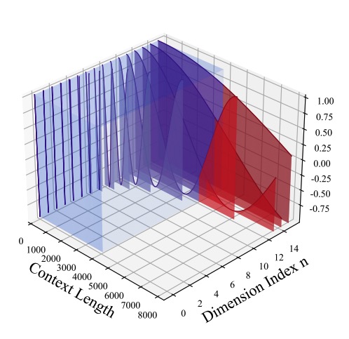
Figure 1. The visualized relationship among the period, training Length, and extrapolation, the periods of dimensions
past the critical dimension (in red) stretch beyond the training context; credited to Liu, Xiaoran, et al., 2023
Now back to NTKRoPE, we’ve concluded that only the last dimension \(d=\frac{\|D\|}{2} - 1\) can expand the wavelength by \(s\), even it doesn’t complete a full rotation (\(2\pi\)). In other words, suppose we have a model pretrained with 512 context length, we want to
expand it to 1024, each head dimension is 64, then only the \(\mathrm{dim}=31\) can ensure all interpolated position ids are just located within the wavelength that are sufficiently trained. Dimensions larger than \(d_{extra}\), however, do not complete a full rotation, and some of their position IDs are located outside the sufficiently trained wavelength, which we denote these position IDs as “out-of-bound” for that dimension.
The farther the dimension deviates from the critical dimension \(d_{extra}\), the more interpolated “out-of-bound” position IDs the dimension have outside the range of its partially trained wavelengths.
What’s even worse, if the period of the signal is longer than the truncation length (max context length for LLM pretraining) in time domain, it means that the signal may not complete a full cycle within the max context. This time domain truncation is equivalent to multiplying the original signal by a rectangular window. In the frequency domain, this is equivalent to convolving the original signal’s spectrum with a sinc function. The sinc function has the property that its main lobe is concentrated at the major frequency, while the side lobes extend outward. Therefore, the energy originally concentrated at a major frequency will spread out to nearby frequencies, a phenomenon known as spectral leakage. Because the energy of the major frequency spreads out to surrounding frequencies, the signal’s energy is “dispersed” across a wider frequency range. This means the dimension beyond \(d_{extra}\) has a low SNR compared to those within the \(d_{extra}\), which makes those dimension even less training.
One possible way to mitigate the “out-of-bound” values is slightly increase the scale value so that more dimensions can ensure the interpolated position ids to locate within the critical dimension.
OR
we do what CodeLLaMA does: scale up the rotation base to 1M.
In conclusion, why could YaRN be the best choice to expand the context?
It is because it fixes the “Out-of-Bound” Problem in a less elegant but more effective way. In YaRN, we manually define upper and lower frequency bounds. These bounds can vary depending on the specific model in use. When dealing with frequencies below the lower bound, we do interpolation. Conversely, for frequencies beyond the upper bound, we apply extrapolation. For frequencies falling within the range between the lower and upper bounds, we apply a combination of both interpolation and extrapolation.
As long as we can find the sweet point low-bound frequency, the “Out-of-Bound” Problem will be effectively solved.
How Mistral solves the long context problem
Mistral first introduced the sliding window in their blog. They claim the sliding window attention mechanism can both save compute cost and expand the context length by stacking layers of transformers.
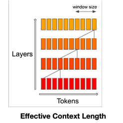
Figure 2. Sliding Window Mechanism (SWM); At each attention layer, information can move forward by W tokens at most: after two attention layers, information can move forward by 2W tokens, etc.
At first glance, it seems that Figure 2 is trying to show me that there exists a layer-wise shifting sliding window that can propogate token information to the next layer so that the context input can be extrapolated very long. However, Figure 2 is just to explain how information propagates along the depth of the network.
The main idea of the sliding window mechanism is to restrict each token to only attend to other tokens within a fixed-size window W. Nevertheless, the propagation of information through the network does not solely rely on the size of the attention window, it also relies on the stacking of multiple attention layers, more like an indirectly access.
For example, we have a sequence of tokens [A, B, C, D, E, F, G, H], and let’s say oursliding window (W) is 3 tokens wide
The output of Layer 1:
Token \(\hat{A}\) integrates information from [A, B, C].
Token \(\hat{B}\) integrates information from [A, B, C, D].
Token \(\hat{C}\) integrates information from [A, B, C, D, E].
Layer 2:
when token \(\hat{A}\) in the second layer attends to token \(\hat{B}\), it’s indirectly also getting information about token D, and when it attends to token \(\hat{C}\), it’s getting information about tokens D and E.
This means token A in layer 2 has a “reach” that extends itself to token E, even though it can only directly attend to [A, B, C].
As for a decoder-only model, the SWM is more straightforward, as tokens can only attend to previous tokens in an auto-regression way.
The output of Layer 1:
Token \(\hat{A}\) integrates information from only A.
Token \(\hat{B}\) integrates from A, B.
Token \(\hat{C}\) integrates from A, B, C
and so on.
After Mixtral-8x7B is released recently, people supersingly find that MoE can magically extend the context length without any interpolation / extrapolation tricks we used in DynamicNTKRoPE, YaRN, etc.
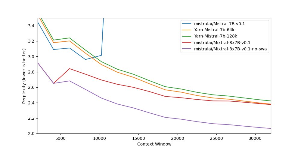 Figure 3. Perplexity evaluation; Mixtral (SMoE) works quite effectively even without the need for any fine-tuning. Moreover, it’s worth noting that disabling sliding window attention can actually enhance model’s the long context ability.
I have to say Figure 3 is hilarious. It shows that extending the context length is only a byproduct of MoE models, yet it still outperforms YaRN-Mistral, which I once bellieve to be the most promising way for manipulating RoPE to expand the context length.
Why it works?
I think it is because every expert is assigned only part of a long token sequence. Imagine there are eight experts simultaneously reading a 1000-token article, with each person assigned a portion of those 1000 tokens. Afterwards, they collaborate to integrate their individual understandings, and that’s how the expansion occurs.
One More Thing (updated on Feb, 2024)
Before Needle-in-a-Haystack test comes out, researchers often use perplexity (negative log-likelihood of the next token) for evaluation. But is it really a reliable metric? Does low loss always mean high retrival performance on long context? The answer is: NO
Chen, Mark, et al. shows us in the paper:
similar test loss could result in substantially different behavior when performing precise retrieval
If you ask me how to expand the LLM context length in Feb, 2024, I will answer you:
Only data matters.
In a word, by continual pretraining with a carefully domain-mixed dataset, and increasing the RoPE base without any modifications such as YaRN, it’s possible to achieve a longer context length than what was initially pre-trained.
Hence, there’s no necessity for further modifications to RoPE. Simply build a carefully curated dataset, inflate your models into MoE, and continue pre-training. These are all steps that’s required to extend the LLM context length. Besides, I think using ‘activate the LLM context length’ to describe the process sounds more reasonable, given that LLMs have already acquired this capability during its pretraining stage.
Just like what Fu, Yao, et al. claims
We hypothesize that the capability to utilize information at arbitrary locations within long context length is (mostly) already acquired during pretraining, even for models pretrained on substantially shorter 4K contexts.
Reference