Background
Inference-time scaling in Large Language Models (LLMs) has been a hot topic recently. The concept of “slow thinking” in LLMs, where more computation during inference leads to significant performance improvements, has received widespread attention and has been proved effective. The open-source community has made significant achievement in reproducing the “slow thinking” approach, milestone works such as Lessons of PRM in Maths, rStar-Math showing us the use of Monte Carlo Tree Rollout methods to iteratively train Process Reward Models (PRM) and synthesize Chain-of-Thought (CoT) data.
But what about the diffusion model? Is it necessary to implement inference-time scaling there as well? And could this be just another story told by NVIDIA for their stock prices?
The answer, in my view, is a definitive “necessary for diffusion model”.
SDE V.S. ODE
In fact, we’ve already seen how inference-time scaling in diffusion models can be beneficial, particularly for the ODE v.s. SDE sampling.
\[dx=-\underbrace{\dot{\sigma}(t)\sigma(t)\nabla_{x}\log p(x;\sigma(t))dt}_{\text{PFODE}}\; \underbrace{-\;\underbrace{\beta(t)\sigma^{2}(t)\nabla_{x}\log p(x;\sigma(t))dt}_{\text{deterministic noise decay}}+\underbrace{\sqrt{2\beta(t)}\sigma(t)dw_{t}}_{\text{noise injection}}}_{\text{Langevin diffusion SDE}}\]
Above equation represent the general form of diffusion sampling. As you can see, sampling consists of two main terms: PFODE and Langevin SDE. The most interesting aspect here is that during noise decay, Langevin Diffusion SDE also injects noise (the third term). This dual role of denoising and noise injection helps mitigate the error caused by pure denoising, effectively creating an inference-time scaling effect by increasing computation.
SiT paper propose a similar conclusion:

Figure 1. The ODE converges faster with fewer NFE, while the SDE is capable of reaching a much lower final FID score when given a larger computational budget
This observation emphasizes an essential trade-off: ODE is computationally cheaper and converges faster, while SDE excels with a larger computational budget, producing more refined results (in terms of FID score). Therefore, while ODE provides faster convergence, SDE’s ability to inject noise in the diffusion process to mitigate accumulated errors during sampling can be computationally scaled up appropriately.
Implications for World Model and Video Generation
I believe that the inference-time scaling in diffusion models is a critical factor in solving issues in world models and video generation models, especially in cases where physical simulation is important. Intuitively, scaling up computations during inference should be beneficial to achieve higher-quality results, since diffusion models can allocate more computations to render complex scenes and simulate complex physics phenomenon.
How Can We Implement Inference-Time Scaling in Diffusion Models?
If inference-time scaling offers benefits in diffusion-based generation, the next question is: how can we implement this in diffusion models?
In fact, this is actually not a simple task. The challenge lies in the principles of Diffusion Models.
Increasing NFE?
Diffusion Models work by denoising, gradually transforming pure noise into an image or video latent feature. Therefore, it seems that inference-time scaling for Diffusion Models should be easy, why not just simply increase the denoising steps? This is often known as increasing the number of function evaluations (NFE). However, many studies have already found that increasing NFEs will soon reach a plateau in the generated image/video quality after a certain number of steps. Therefore, merely increasing the NFE is not a viable approach.
DPO for Diffusion?
Although there have been methods like SD + DPO, DPO’s reward is calculated at the instance level through preference pair data. Whether for images or videos, this level of granularity is too coarse. Coarse-grained rewards struggle to improve training data efficiency, and the model can easily “hack” preference data. This makes preference data challenging to work with. At least, making a preference data for images is one thing, but what about videos? Can we really have a clear preference between frames of two videos?
PRM + MCT rollout like what LLM does?
Then, Could we just follow LLMs using PRM + MCT rollout? As of the time I’m writing this blog (Jan 18th, 2025), the answer seems to be no.
Unlike LLMs, where generation happens with discrete tokens, most diffusion models generate in a continuous space. This makes applying PRM + MCT rollout methods to diffusion models infeasible. We cannot create CoT-like data for training diffusion models in the same way we do with text modalities, because images and videos are not discrete tokens. Actually, we even have no idea what CoT-like data shoule be like for diffusion model. We can’t extend CoT chains, manually set terminal points, calculate terminal rewards, and then use various rules to roll the data.
Of course, one path could be to drop the continuous latent space of diffusion models and switch to a discrete latent space and use AR (autoregressive) generation for images and videos. Once generation becomes a token-by-token process, all of the LLM’s RLHF methods become applicable.
In this area, I think NVIDIA’s Cosmos-1.0-Autoregressive has made the most solid advancements.
Cosmos-1.0-Autoregressive has explored extensively and gained many insights into design.
First, the key challenge of training an image/video generation in AR fashion is how to develop a tokenizer with sufficient spatial-temporal compression.
Cosmos uses a discrete tokenizer of 8x16x16, but this compression rate still seems inefficient. The sequence length of high-resolution images and long videos with such a tokenizer will become extremely long, even longer than the training context length that has been validated for text modalities. A natural follow-up is to pursue a tokenizer with even higher compression, such as 16x32x32. However, the Cosmos team considers 8x16x16 to be already quite aggressive.
“As a result of aggressive compression, it could sometimes lead to blurriness and visible artifacts in video generation, especially in the autoregressive WFM setting, where only a few integers are used to represent a rich video through discrete tokenization.”
Thus, they had to design a diffusion decoder, where discrete token video is treated as the conditional input to the denoiser. The final image/video output is then generated by the diffusion decoder.

The upper bound of this approach is clear. It depends on the quality and compression rate of the tokenizer, but it still doesn’t drop the continuous space for generation. After all, images and videos are inherently continuous modalities. Furthermore, the long sequence lengths far exceed those of text, which poses a significant challenge for training infrastructure perspective, not even mention serving such a model.
Search Noise and Path
On January 17th, 2025, DeepMind published a paper on scaling Diffusion Models. The paper proposes what seems to be the most promising approach up till now.
-
Rollout Initial Noise, referred to as Zero-Order Search, uses verifiers’ feedback to iteratively refine noise candidates.
-
Search over Paths, which leverages verifiers’ feedback to iteratively refine diffusion sampling trajectories.
The paper also introduces, for the first time, a mechanism similar to PRM within the entire pipeline, referred to as the verifier. These verifiers are classifiers trained based on CLIP and DINOv2, which use class label logits to help roll out the Initial Noise and Search over Paths. However, this rollout pipeline is still in its very early stages. The search algorithm is quite easy to hack via the reward verifier.
From my understanding, although Rollout Initial Noise has some solid theory behind it, as many studies have shown that certain good noise do exist for better generation results. However, no single configuration is universally optimal.
What a RLHF For Diffusion should be like?
Upon reviewing it again, the problems that need to be solved to run RLHF for the diffusion model are:
-
How to define process rewards in continuous space?
-
How to enable the diffusion model to self-improve, similar to how LLMs perform data rollouts based on MCT?
-
What exactly does the diffusion process reward model look like?
Below, I propose a method I believe to be feasible.
The current flow-matching method actually starts by randomly initializing noise and letting the model fit the distribution of training data to construct a vector field. This vector field pushes the initial noise towards the expecting results. Interestingly, in robotics path planning, similar algorithms have existed for a long time, and they are called potential fields.
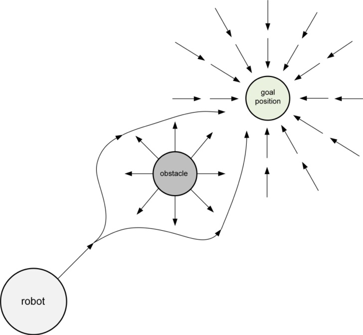
Figure 2. potential field for robot path planning.
When you examine potential fields, you’ll find many similarities with flow matching. In potential fields, the robot is regarded as a positive charge, and the goal as a negative charge, with opposite charges attracting each other, creating a potential field that guides the robot’s path planning.
However, in the real world, physical obstacles exist. To avoid obstacles, robot often regard obstacles as positive charges, like the robot itself, so that positive charges repel each other, and negative charges attract.
Now you see the inspiration: The current diffusion training only considers the start and end points, without considering obstacles along the probabilistic path. These obstacles should be human preferences. For example, when generating a video, if a person walks through a wall, this breaks physical laws, and thus the obstacle represents physical law. Similarly, if an image generates a person with six fingers, the obstacle represents human preferences.
Therefore, in continuous space, the process reward should be:
\[x_{t-1} = U_{\text{att}}(x_t, t) + U_{\text{rep}}(x_t, t)\]
where \(x \in [0, 1]\)
\(U_{\text{att}}\) is the “attractive” vector field, move the initial noise \(x_1\) to the goal \(x_0\)
\(U_{\text{att}}\) is the “repulsive” vector field, make the initial noise \(x_1\) avoid obstacles.
Thus, the process reward in continuous space should be such that when the probabilistic path approaches obstacles, it is repelled by them. This repulsion force should have a threshold, Q∗, which represents the process reward score that needs to be searched via RLHF.

Figure 3; Repulsive by Obstacles then point locates inside \(Q^*\)
More specifically, this process reward score should be: when a denoising step hits an obstacle/locate inside the $Q^*$, the model should “feel the pain” and revert to the previous step, continuing to search for a collision-free path.
This is similar to search over paths and also shares similarities with the Langevin dynamics term in SDEs. The algorithm for search over paths is as follows:
Step 1: Sample N initial i.i.d. noises and run the ODE solver until a certain noise level \(σ\). The noisy samples \(x_σ\) serve as the starting point for the search.
Step 2: Sample M i.i.d. noises for each noisy sample and simulate the forward noising process from \(σ\) to \(σ+Δf\) to produce \(x_{σ+Δf}\) with size M.
Step 3: Run the ODE solver on each \(x_{σ+Δf}\) to the noise level \(σ+Δf−Δb\), obtaining \(x_{σ+Δf−Δb}\). Run verifiers on these samples and keep the top N candidates. Repeat steps 2-3 until the ODE solver reaches \(σ=0\).
Step 4: Run the remaining N samples through random search and keep the best one.
However, Langevin dynamics does not well incorporate a repulsive potential; it’s more focused on random search. Search over paths relies on verifiers to provide process rewards, but verifiers are vulnerable and can be easily “hacked” by the model.
Thus, I propose the following process reward:
\[U_{\text{rep}}(q) = \left\{\begin{array}{ll}\frac{1}{2} \eta \left( \frac{1}{D(x_t, t)} - \frac{1}{Q^*} \right)^2, & D(x_t, t) \leq Q^* \\0, & D(x_t, t) > Q^*\end{array}\right.\]
where \(D(x_t, t)\) is the distance from the noisy latent feature \(x_t\) to the obstacles under the vector field.
We assume that such a vector field, combining both attractive and repulsive fields, has already been learned through the training data. For the diffusion model, this allows it to self-improve, similar to how LLMs perform data rollouts based on MCT—constantly starting from random points in latent space to search for the best collision-free probabilistic path.
Now, the key question is: how do we represent these obstacles in latent space? In other words, what exactly does the diffusion process reward model look like?
When we lack ideas, we can look at how robotics addresses this problem.
Configuration Space
Firstly, robotics path planning is not always done in Cartesian space. Some method does path planning in a configuration space.
What is a configuration space?
The space of all configurations is the configuration space or C-space.
— C-space formalism: Lozano-Perez ‘79

For a robot with two degrees of freedom, \(\alpha\) and \(\beta\), the space defined by these two variables is the robot’s C-space \(C_{\text{robot}} \in\mathbb{R}^2\). Each degree of freedom theoretically spans \([0,2π]\), but due to physical constraints, \(\alpha \in [0,\pi]\) and \(\beta\in [0,2\pi]\). In \(C_{\text{robot}}\), each point represents a robot’s pose configuration. Points that do not satisfy physical laws, or where the robot hit itself, are termed singularity points. All singularity points form the singularity space.
Therefore, moving collision-freely from pose A to pose B in the configuration space becomes a simple point-to-point path planning problem. The space of poses that cause collisions constitutes the obstacles in C-space.
You may notice that there’s an amazing similarity between C-space and VAE. Both serve as compressed spaces, translating a higher-dimensional path planning problem into a lower-dimensional one. Also, it’s common knowledge that VAE’s dimensionality is generally not large. Even in temporal and spatial compression, such as 8x16x16, the latent dimension typically remains small (e.g., 8, 12, 16). One reason is that increasing the latent dimension adds redundancy in the latent space, making DiT learning harder. Although scaling up DiT parameters can somewhat mitigate the redundancy of larger latent dimensions, most developers don’t follow this practice.
This can be verified in C-space: as a robot’s degrees of freedom increase, the C-space’s dimensionality increases, and so does the singularity space. This is why VAE redundancy increases when latent dimension increases.
Semantic VAE
Returning to obstacle representation, we can follow how C-space represent obstacles. By projecting data or concepts that do not align with human preferences into the VAE space, we can guide the initial noise to avoid falling into singularity or collision spaces. This is what we call rollout initial noise, also known as zero-order search.
Thus, a promising future research for optimizing VAEs seems clear: make the VAE latent features not just a compressed space, but also introduce semantics to align with them. This way, we can project human preferences and physical laws into the VAE latent space, similar to how obstacles are represented in C-space.
Fortunately, some papers have already taken this approach. For example, Reconstruction vs. Generation demonstrates that by introducing DINOv2, the latent space not only learns more efficiently but also lays the foundation for expressing human preferences and physical laws in the future.
 Figure 4. The latent space learns more efficiently by aligning DINOv2
Thus, if self-supervision vision foundation models can serve as a bridge for reconstruction and representation, we can project more obstacles into the VAE space and even directly use this feature as a classifier to learn human preferences.
Conclusion
For the diffusion model, when doing Process Reward in continuous space, we can reference the robotics potential field method. We treat the initial noise as a positive charge, the generated target as a negative charge, and introduce obstacles as positive charges. The repulsive vector fields between the positive charges and the attractive vector field between the positive and negative charges should be superimposed to search for the strength and effective range of the repulsive vector field of each obstacle.
To achieve this, we need to align the VAE with world knowledge, allowing us to construct obstacles in the VAE space by inputting text, images, or videos. At the same time, the VAE features should ideally integrate reconstruction and representation. By training a large number of human preference classifiers, we can build an effective search space within the VAE space.