TL; DR
Let us first imagine we are under an unknown latent feature space. We begin at a randomly initialized point sampled from a normal distribution, and our goal is to somehow reach the target that aligns with human preferences, regardless of what the target is—could it be a sequence of words, an image, or a video. This is undoubtedly a path planning problem. Today, we already have algorithms including the Large Language Model (LLM) and Diffusion Models to navigate us toward the target, whether through next-token prediction or denoising.
If we take all generative tasks as path-planning tasks, we can explain many empirical results.
Less is More?
LIMA emphasizes that data quality is more important than quantity, which has now become common knowledge in the community. But why is this the case? Returning to our path-planning analogy, we can notice that defining a clear goal is really hard since human preferences are diverse and complex. High-quality data, however, provides a clearer and more specific target, enabling models to chart a more precise path. On the other hand, a large volume of low-quality data can only lead to ambiguous objectives which makes the learning process far less efficient.
Accelerate Generation
Following the analogy above, in language models, the starting point is the context from the input prompt, where each token represents a step toward the goal of aligning with human preferences or world knowledge. Similarly, in diffusion models, the starting point is a Gaussian noise sample mapped to the latent feature space, and each denoising step is a step toward aligning with the intended features.
Accelerating inference can be thought of as taking multiple steps at once. There’s ongoing research exploring this concept. For example, in language models, lookahead decoding introduces an N-Gram Pool to address the limitations of Jacobi iteration, where generation can often go wrong because of multiple steps once. Similarly, CLLMs fine-tune LLMs to generate n-tokens in parallel, mimicking autoregressive decoding. They simplify this by mapping the randomly initialized states to intermediate points on the Jacobi trajectory.
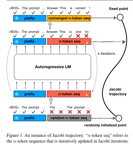
Figure1. Image Credit to CLLMs
In image/video generation, this idea is also known in techniques like Flow Matching and its optimal transport variant, Rectified Flow.
Suppose the goal distribution \(P_1\) represents human-aligned preferences. Flow Matching suggests that instead of modeling the goal distribution, we should model the vector fields that define a probability density path that pushes an initial point sampled from a Normal distribution \(P_0\) toward the goal distribution \(P_1\).
Let \(p\) denote a sample drawn from the distribution \(P\); \(t\) represents the intermediate state transitioning from the normal distribution to the goal distribution.
In contrast, Diffusion models start with data points and gradually add noise until it approximates pure noise. The models are then trained to predict the noise added at each timestep \(t\).
During inference, iddpm is more like a stochastic process, where \(p_0\) takes random steps toward \(p_1\), which explains why it typically requires many steps (~100) to produce a satisfactory output. DDIM, however, addresses this by introducing \(p_{1|t}\) to calibrate its path.
The overall process can be summarized as follows, where \(h\) is the step size:
\[p_t \Rightarrow \epsilon_t \Rightarrow p_{1|t} \Rightarrow \mu(p_t, p_0) \Rightarrow p_{t+h}\]
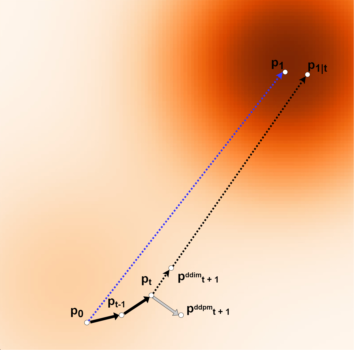
Figure 2; \(p_0\) is a sample from a Normal distribution \(P_0\), while \(p_1\) is a sample from the target distribution \(P_1\). In the inference stage, the denoising process can be viewed as a path-planning problem. At timestep \(t\), we denoise the pure noise \(p_0\) into \(p_t\).
The key question is: what should the next step be?
Since DDPM is like a stochastic process, the step at \(t+1\) could completely diverge from \(p_1\). However, DDIM calibrates this process by \(p_{1 | t}\).
The next step is constrained to locate along the line between \(p_t\) and \(p_{1∣t}\), therefore making a more stable and directed generation. (See the Appendix for the mathematical proof.)
Even though \(p_{1∣t}\) predicted by neural networks may not be accurate to the ground truth goal point \(p_1\), it still can be a useful guide for the next move. This is why DDIM can accelerate the generation process compared to DDPM.
Rectified Flow, however, optimizes the denoising process by learning the ODE to follow the straight paths connecting the initial points to the goal point, see the blue dotted line in Figure 2. This simple and intuitive path is the optimal path that can be generated with only one step. I strongly recommend you read the Flow Matching paper. There is a counter-intuitive phenomenon that while video/image generation is inherently more complex than text generation, models for generating images and videos typically have far fewer parameters than language models. Additionally, they often do not require post-training processes like PPO (Proximal Policy Optimization) or DPO (Direct Preference Optimization). I believe the key point of this is that image and video generation models learn how to represent vector fields, allowing them to generate complex outputs with fewer parameters compared to language models.
In contrast, language models trained with auto-regressive loss focus primarily on modeling the target distribution \(P_1\). However, they do not inherently learn efficient and stable path planning to reach a desired output. This inefficiency makes the language model waste too many parameters to memorize all samples within \(P_1\) from tons of training tokens. Algorithms like PPO and DPO are necessary for language models because these algorithms aim to teach the model how to plan more efficiently and stably through reinforcement learning. Notably, PPO enables token-level optimization, whereas DPO does not.
Why do hallucinations happen?
In a recent study by Gekhman, Zorik, et al., the authors reveal that supervised
fine-tuning (SFT) struggles to integrate new knowledge into a Large Language Model (LLM). The authors propose an approach by categorizing fine-tuning datasets into four categories as below:

Figure 3. Knowledge Categories
Their findings suggest that the most effective fine-tuning datasets should consist of HighlyKnown, MaybeKnown, and WeaklyKnown data, with a minimal amount of Unknown data.
This conclusion makes me rethink what is SFT inherently.
From Denosing Perspective
To simplify the problem, let’s take LLMs as a linear system. Under this assumption, We define \(A\) as the weight matrix of multiple transformer blocks, while \(x\) and \(b\) represent input embeddings and text hidden features, respectively. We link autoregressive generation to the denoising process:
\[A \cdot [x_{bos}; x_{prefill}; x_{gen}^{\prime}]\]
As for the input embedding \(x\), since the \(x_{gen}\) is unknown yet, we initialize it randomly as \(x_{gen}^{\prime}\)
During SFT LLM, we try to solve the following equation:
\[A \cdot [x_{bos}; x_{prefill}; x_{gen}^{\prime}] = [b_{prefill}; b_{gen}; b_{eos}]\]
Here is an intriguing question: if the linear equation has no solution, can fine-tuning still be effective?
A Hypothesis:
-
If \(Ax=b\) has no solution, it is exactly the Unknown case mentioned
in Gekhman, Zorik, et al. Since we expect LLM always responses, it has to hallucinate with an approximate solution to \(Ax=b\) and this is where hallucination happens.
-
If \(Ax=b\) has a unique solution, it links to the HighlyKnown when Greedy decoding always predicts the correct answer
-
If \(Ax=b\) has infinitely many solutions, it relates to MaybeKnown or WeaklyKnown instances when Greedy decoding sometimes predicts the correct answers.
This hypothesis explains why hallucination happens: it is when \(Ax=b\) has no solutions but we force the LLM to return us an approximate solution.
From Path Planning Perspective
Appendix